Blackstar: raytracing black holes with Haskell
General relativity is cool. Some of the ideas introduced there are conceptually so simple and beautiful that I can’t help but appreciate Einstein’s work.
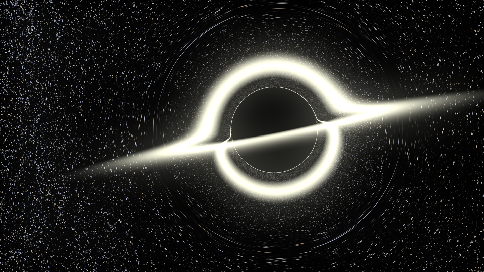
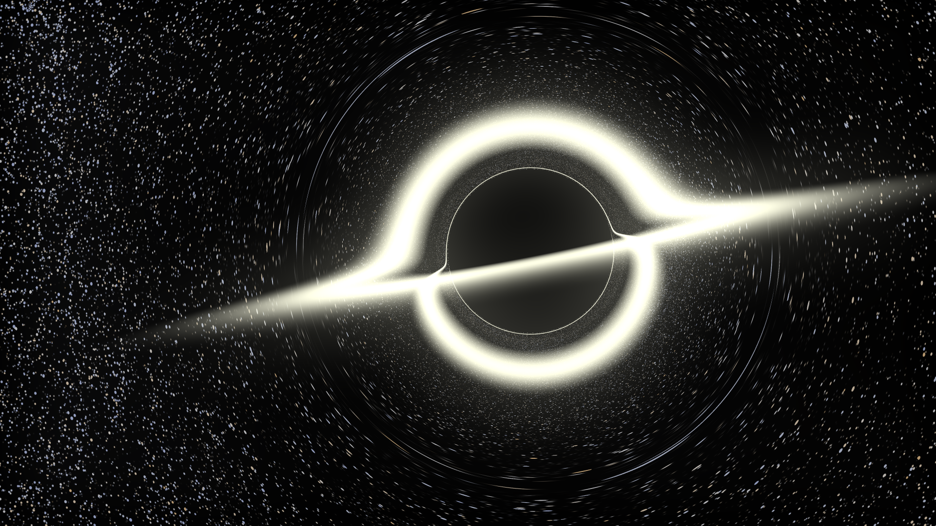
When I saw Interstellar in 2014, I was especially amazed by the black hole, Gargantua, that they had rendered. There’s no doubt the artistic license was extensively used there, but still, they used the Kerr metric to describe a spinning black hole and even published a scientific paper about it.
Then, a few months later, rantonels’ excellent article and Python code appeared on Hacker News. He was rendering a Schwarzschild black hole by means of ray tracing, making clever use of NumPy for fast calculations. You should definitely check out the article and the code — they’re awesome and you’ll most likely learn a lot!
As a numerical physics enthusiast, I began wondering if I could render such images myself. By the time, however, I wasn’t skilled enough in general relativity to grasp the theoretical side. I then noticed there was going to be a general relativity course held at the university next year. I decided to wait until that.
The course began and the patient waiting paid off. Soon enough I noticed the simplicity of the core ideas like geodesics, which were necessary to do this kind of a simulation. I immediately began coding the ray tracer, and here I am, three weeks later, writing an article about the finished code: Blackstar. Later on, the project was discussed on r/haskell and Hacker News.
As an acknowledgement I’d like to note that my code owes its existence to rantonels’ work. You’ll most likely notice some evident similarities between these two projects. However, there are also some differences, and I think Blackstar ended up as a project in its own right. For one, I decided to implement the whole thing in Haskell, given that I had just studied two courses of it. This project turned out to be a great way to learn more about Haskell.
Schwarzschild geodesics
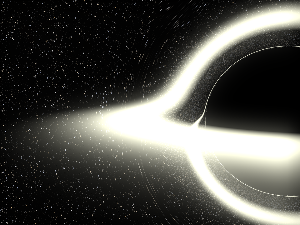
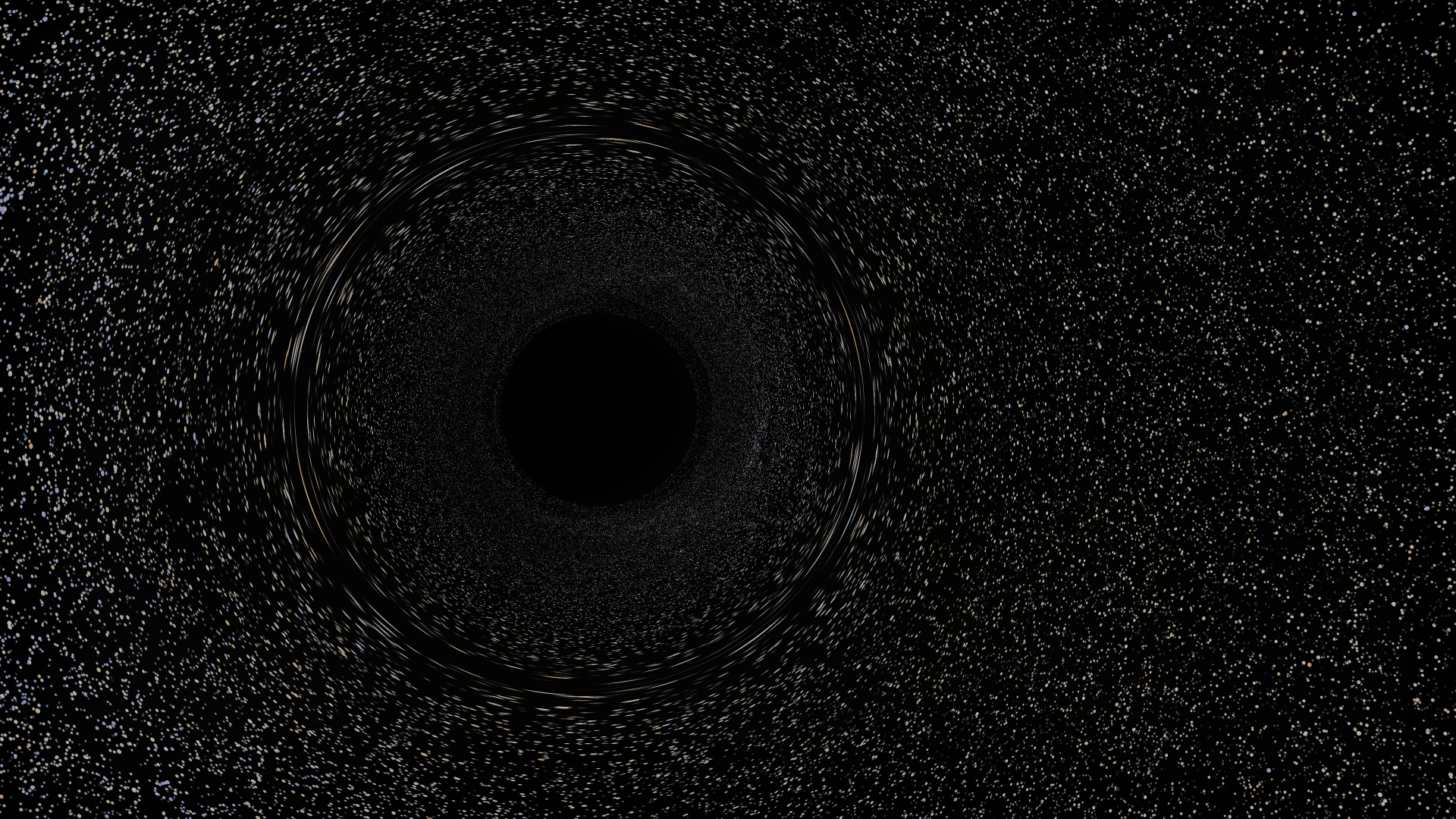
What do we need to visualize the gravitational lensing effect produced by a dense object such as a black hole? In Newtonian mechanics, massless particles like photons move in straight lines. In general relativity, the huge mass density of a black hole generates spacetime curvature. The generalization of a straight line to a curved spacetime is a geodesic — it turns out that photons move along geodesics, which are some curved paths.
The spacetime curvature caused by a non-rotating black hole is described by the Schwarzschild metric. In principle, one would have to solve a system of four differential equations — the geodesic equations — to get the geodesics. I tried this first as I wanted to go the “fundamental route”, but I only ended up struggling with singularities at the poles of the spherical coordinate system. It could still almost work fine, except for some black points in the image where divergence occurred.
In the end, however I decided to take the same route rantonels had taken: take advantage of the symmetries of the Schwarzschild spacetime to derive much simpler (and, most importantly, non-singular) “equations of motion” for the photons. The derivation (the most of it) can be most likely found in any decent GR textbook. However, I decided to write a little article about it in order to give people with no GR background a possibility to understand some of the beautiful concepts of general relativity. You should check it out! Alternatively, see rantonels’ two articles for a slightly different take on the derivation.
After the theoretical work, the ray tracing boils down to just solving the three-dimensional Newton’s equation of motion \[ \ddot{\mathbf{r}} = -\frac{3}{2} h^2 \frac{\hat{\mathbf{r}}}{r^4} \] with fourth order Runge-Kutta. Here \(\mathbf{r}\) is the three-dimensional Cartesian position vector, \(r\) its norm, \(\ddot{\mathbf{r}}\) the acceleration and \(h\) the “angular momentum” of the test particle. The details have been covered in my article.
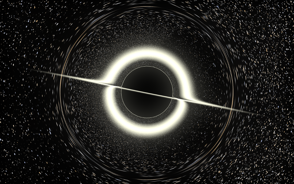
The accretion disk
Unlike the geodesics, there isn’t much physics to the accretion disk. Its main function is to provide some Interstellar-esque eye candy. It is modeled as an annulus with zero thickness. The light emitted by the disk is monochromatic, chosen by some HSV value. The opacity \(\alpha\) is taken from a “density function”. I tried out a couple of possible density profiles, ending up with one expressed in terms of the radius \(r\): \[ \alpha(r) = \sin \left[ \pi \left( \frac{R_\text{outer} - r}{R_\text{outer} - R_\text{inner}} \right)^2 \right], \] where \(R_\text{inner}\) is the inner radius of the disk and \(R_\text{outer}\) the outer one. This gave the disk a nice plasma-like look and was my fair share of artistic license.
Haskell appreciation
During the project, I had to code a good variety of actions from config file parsing and data structure serialization to quick, parallel computations. I was delighted to realize there’s a good selection of high quality packages available for pretty much every action I wanted to implement. In addition, almost all of them were pretty well documented. I’ve listed some particular cases below.
The tooling has also gone a long, long way, primarily thanks to stack and LTS Haskell. stack makes the installation of the toolchain and the dependencies really easy — I could painlessly do it even on Windows 10 (and it was fast!)
Parallel ray tracing with repa
By its nature, the ray tracing is a highly parallelizable process: the light rays don’t interact with each other in any way, so there’s no shared state between threads. There are a couple of options for implementing such parallel computations in Haskell. I was torn between repa, which seems to be the de facto choice for high performance computations, and friday, a pretty fresh library specializing in image processing with an interface similar to repa.
friday was chosen for the initial implementation. Saving images to PNG files was implemented with friday-devil. It was certainly a pleasure to work with. Given the nice interface and some handy colour space conversion functions, the image processing was really easy to implement. Thanks to DevIL, file saving was lightning fast.
However, a couple of things made me switch to repa and JuicyPixels in the end. The main reason for this was to keep the dependencies strictly Haskell-only. This way building Blackstar would be just one stack build away, without the need to worry about extra C dependencies. As a bonus, these libraries had the convenience of being readily available in LTS Haskell (although this is not a big deal when using stack).
That said, friday is still a great library and I’ll be happy to use it for future image processing projects depending on the project’s requirements. There’s also friday-juicypixels in development, possibly allowing image file I/O based on JuicyPixels in the future.
Starry skies with kdt
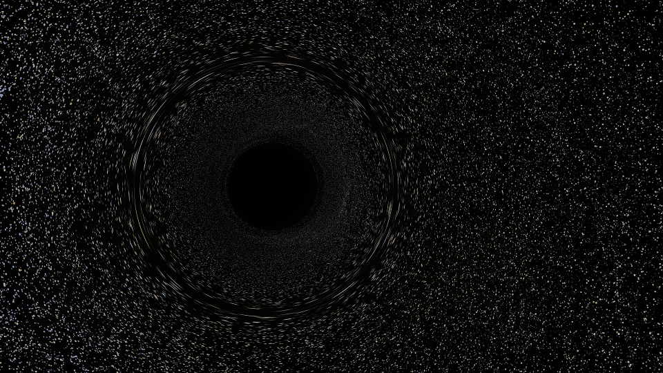
When some “sight ray” in the ray tracing travels far enough from the black hole, the colour of the corresponding pixel is sampled from the celestial sphere — whether the ray came from a black part of the sky or a star.
I decided to make use of some star catalog data. In these star catalogs, the positions of the stars are listed along with their apparent magnitudes and spectral types — just enough to create a visual representation of the celestial sphere.
Sampling stars from a list of several hundred thousand stars is obviously not going to be fast. To tackle this, I first converted the position data (two angles parametrizing the celestial sphere) to three-dimensional unit vectors. This makes it easy to compare them with the direction vectors of the rays leaving to infinity. Second, I decided to order the stars into a k-dimensional tree for faster lookups. There are several k-d tree implementations available on Hackage. I settled for kdt, which looked simple, flexible and stable.
The construction of the k-d tree of \(n\) stars is approximately a \(\mathcal{O}(n \log n)\) operation, and in practice it took about half a minute on my computer. It’s a one time thing, so I didn’t definitely want to do it every time the program was run. I decided to use cereal to serialize the tree and save it to a file in binary form. The datypes in kdt didn’t directly lend themselves to serialization: I had to fork kdt and expose some of the datatypes in order to derive the Serialize typeclass for them. However, this wasn’t a very big deal. Stack made it very easy to use the fork instead of the official package in LTS Haskell. If you know how to work around this without modifying the package, please contact me!
EDIT: The maintainer of kdt kindly upgraded the upstream package to make the necessary types visible. The fork is not required any more.
Experiment: automatic differentiation
When starting this project, I had a pretty ambitious idea in my mind. The most general way to do ray tracing in Riemannian geometry is to let the user supply the spacetime metric to be used. From there, one can compute the Christoffel symbols and express the geodesic equations in terms of them. Computing the Christoffel symbols involves differentiation of the metric components. Depending on the complexity of the metric, these expressions can get quite cumbersome and at least very tedious to type in.
I began wondering if I could work around the problem by employing automatic differentiation (AD). It is an ingenious way to computationally obtain the analytic value of the derivative of a given expression. The method is based on operator overloading and the chain rule of differentiation. By letting the computer calculate the derivatives, exploring more complex metrics could become easier. In Haskell, things like this are fairly easy to implement, thanks to the flexible typing system. An especially good-looking implementation is the package ad, which seems exceptionally versatile and well-made.
However, nothing comes for free. In a computationally expensive application like this, it quickly became obvious that the automatic differentiation had quite an impact on the execution time. In my early tests, I saw a difference of two orders of magnitude between the explicit Schwarzschild geodesic equations and the ones obtained by AD. You can find the AD work in a branch of my repo.
ad is still an amazing package, and I intend to use it in the future for some computationally less intensive applications. In a highly intensive task like this, one just has to squeeze out every possible bit of speed.
EDIT: Edward Kmett, the creator of the ad package noted on reddit that a better approach would be to compile the expressions derived by ad into machine code. I’m very interested in this idea and intend to try it in the future. It might take some time, though.
Optimization (help wanted!)
Speaking of speed, this project was really the first number crunching project I have done in Haskell. Other than the optimization tips given for Repa, I didn’t do much in order to optimize the code. It seems to be reasonably speedy, though.
For similar upcoming projects, I’d love to learn a bit more about writing performant Haskell code. I’m slowly reading up on GHC and performance optimization. If you happen to spot some optimization opportunities in the code, please contact me on GitHub!
